Data Viewer

Important

This section assumes that the reader is already familiar with Application Settings.

Introduction

By default, the data viewer in specvizitor is configured to display the Grizli data products. Specifically, it is using data from the following files:

File	Description
*1D.fits	1D spectrum
*stack.fits	2D stacked spectrum of all exposures
*full.fits	Various extraction products including emission line maps and image cutouts

However, specvizitor’s capabilities go far beyond this. By modifying the data_widgets.yml file, you can create a custom widget configuration tailored to practically any spectroscopic dataset. In this section, you will learn how to configure data widgets in specvizitor, starting with small tweaks to the default configuration and finishing with a configuration “from scratch”.

Configuring the default widgets

Let us start with some examples of how you can configure the default data widgets.

Changing the redshift range

In data_widgets.yml, navigate to plots ‣ Spectrum 1D ‣ redshift_slider ‣ max_value:

...
plots:
  Spectrum 1D:
    ...
    redshift_slider:
      ...
      max_value: 10

Set max_value to any redshift you think would suffice to classify even the most distant objects included in your sample. Next, make the same changes to the redshift slider under images ‣ Spectrum 2D:

images:
  ...
  Spectrum 2D:
    ...
    redshift_slider:
      ...
      max_value: 10

This is required because Spectrum 1D and Spectrum 2D share the same redshift. Once you have made the changes, save data_widgets.yml and launch specvizitor. The maximum value of the redshift slider should be updated accordingly.

Changing the color bar range

Note

This example demonstrates how to change the color bar range of Spectrum 2D, however the same applies to any widget in the images category.

In data_widgets.yml, navigate to images ‣ Spectrum 2D ‣ color_bar ‣ limits:

images:
  ...
  Spectrum 2D:
    ...
    color_bar:
      ...
      limits:
        min: -0.015
        max: 0.015
        type: user

Here, you can set the min and max parameters of the color bar. Once you have made the changes, save data_widgets.yml and launch specvizitor. The color bar range in Spectrum 2D should be updated accordingly.

Linking widget elements

Note

This example demonstrates how to link plot axes, however the same applies to sliders and color bars.

In data_widgets.yml, navigate to images ‣ Line Map 1 ‣ x_axis ‣ link_to:

images:
  ...
  Line Map 1:
    ...
    x_axis:
      link_to: null

Set link_to to Image Cutout. Once you have made the changes, save data_widgets.yml and launch specvizitor. The y-axis of Image Cutout and Line Map 1 should be linked together.

Hiding widget elements

Note

This example demonstrates how to change the visibility of plot axes, however the same applies to color bars, sliders, spectral lines, and widgets themselves.

Tip

Most of the widget elements can be hidden simultaneously by pressing H.

In data_widgets.yml, navigate to images ‣ Spectrum 2D ‣ x_axis ‣ visible:

images:
  ...
  Spectrum 2D:
    ...
    x_axis:
      visible: true

Set visible to false, save data_widgets.yml and launch specvizitor. The Spectrum 2D’s x-axis will disappear from the view.

Adding new widgets

Let us continue with some examples of how you can add new widgets to the data viewer.

Widget types

There are two types of widgets that can be added to the data viewer — images and plots:

images:
  ...
plots:
  ...

Both images and plots can comprise multiple items:

images:
  Image:
    ...
  Spectrum 2D:
    ...
plots:
  Plot:
    ...
  Plot 2:
    ...
  Another Plot:
    ...

Important

All widget names must be unique.

The difference between images and plots lies in the parameters that widgets of these types can have. For example, the color_bar parameter is unique to widgets listed in images, and the plots parameter is unique to widgets listed in plots.

Adding an image

This is a minimal example of data_widgets.yml comprising a single image:

images:
  Image Cutout:
    data:
      filename_keyword: stack.fits

Here, by specifying the filename_keyword parameter, we tell specvizitor to search for files whose filenames include stack.fits. For example, if we load the dataset from the tutorial (see Getting started), specvizitor will discover the following files:

alt_16605.stack.fits
alt_26932.stack.fits
alt_34927.stack.fits

and select one of them depending on the ID of the current object.

Sometimes a FITS file contains multiple images (tables). By default, specvizitor loads the first image (table) from such files. To load a different image (table), we can specify the extname and extver parameters in loader_params:

images:
  Image Cutout:
    data:
      filename_keyword: stack.fits
      loader_params:
        extname: SCI
        extver: F356W

Finally, it is often useful to configure the default range of the color bar attached to the image:

images:
  Image Cutout:
    data:
      filename_keyword: stack.fits
      loader_params:
        extname: SCI
        extver: F356W
    color_bar:
      limits:
        type: user
        min: -0.015
        max: 0.015

Here, type mimics the types of images limits used in SAOImage DS9 and can be either user (in which case it is necessary to specify min and max), minmax (the default value), or zscale.

Adding a plot

Similarly to images, this is a minimal example of data_widgets.yml comprising a single widget for displaying plots:

plots:
  Spectrum 1D:
    data:
      filename_keyword: 1D.fits

Next, we need to specify the plot(s) that will be shown in this widget:

plots:
  Spectrum 1D:
    data:
      filename_keyword: 1D.fits
    plots:
      flux:
        x: wave
        y: flux

Here, wave and flux refer to the columns of a table loaded from the FITS file.

In addition, we might want to configure the plot limits:

plots:
  Spectrum 1D:
    data:
      filename_keyword: 1D.fits
    plots:
      flux:
        x: wave
        y: flux
    y_axis:
      limits:
        min: -0.5
        max: 1.5

Finally, let us add a redshift slider to the widget and make spectral lines visible in the plot:

plots:
  Spectrum 1D:
    data:
      filename_keyword: 1D.fits
    plots:
      flux:
        x: wave
        y: flux
    y_axis:
      limits:
        min: -0.5
        max: 1.5
    redshift_slider:
      visible: true
      max_value: 10
      step: 1.0e-6
      catalog_name: redshift
      show_text_editor: true
      show_save_button: true
    spectral_lines:
      visible: true

A full example

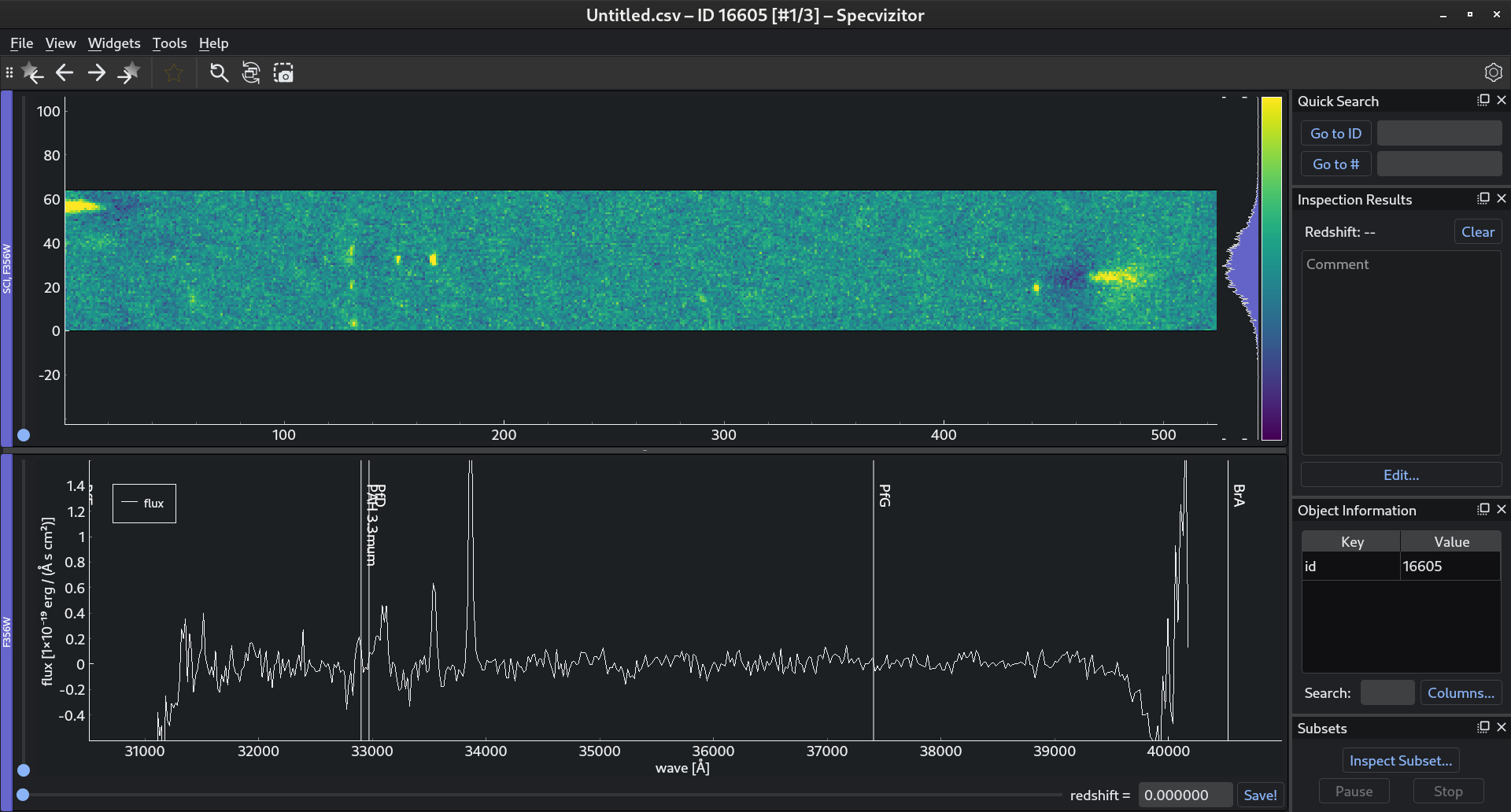
This is a full example of data_widgets.yml which combines the two previous examples:

images:
  Image Cutout:
    data:
      filename_keyword: stack.fits
      loader_params:
        extname: SCI
        extver: F356W
    color_bar:
      limits:
        type: user
        min: -0.015
        max: 0.015
plots:
  Spectrum 1D:
    data:
      filename_keyword: 1D.fits
    plots:
      flux:
        x: wave
        y: flux
    y_axis:
      limits:
        min: -0.5
        max: 1.5
    redshift_slider:
      visible: true
      max_value: 10
      step: 1.0e-6
      catalog_name: redshift
      show_text_editor: true
      show_save_button: true
    spectral_lines:
      visible: true

If you load this file in specvizitor (Widgets ‣ Restore…), you should see the following:

Note

The widget configuration used in specvizitor by default is available here.

Templates

TBU